Equidistributed sequence

In mathematics, a bounded sequence {s₁, s₂, s₃, …} of real numbers is said to be equidistributed, or uniformly distributed, if the proportion of terms falling in a subinterval is proportional to the length of that interval. Such sequences are studied in Diophantine approximation theory and have applications to Monte Carlo integration.

1 Definition
- 1.1 Discrepancy
- 1.2 Equidistribution modulo 1
2 Examples
3 Properties
4 Metric theorems
5 Well-distributed sequence
6 See also
7 References
8 External links

Definition

A bounded sequence {s₁, s₂, s₃, …} of real numbers is said to be equidistributed on an interval [a, b] if for any subinterval [c, d] of [a, b] we have

$\lim_{n\to\infty}{ \left|\{\,s_1,\dots,s_n \,\} \cap [c,d] \right| \over n}={d-c \over b-a} . \,$

(Here, the notation |{s₁,…,s_n }∩[c,d]| denotes the number of elements, out of the first n elements of the sequence, that are between c and d.)

For example, if a sequence is equidistributed in [0, 2], since the interval [0.5, 0.9] occupies 1/5 of the length of the interval [0, 2], as n becomes large, the proportion of the first n members of the sequence which fall between 0.5 and 0.9 must approach 1/5. Loosely speaking, one could say that each member of the sequence is equally likely to fall anywhere in its range. However, this is not to say that {s_n} is a sequence of random variables; rather, it is a determinate sequence of real numbers.

Discrepancy

We define the discrepancy D(N) for a sequence {s₁, s₂, s₃, …} with respect to the interval [a, b] as

$D(N) = \sup_{a\le c\le d\le b} \left\vert \frac{\left|\{\,s_1,\dots,s_N \,\} \cap [c,d] \right|}{N} - \frac{d-c}{b-a} \right\vert . \,$

A sequence is thus equidistributed if the discrepancy D(N) tends to zero as N tends to infinity.

Equidistribution is a rather weak criterion to express the fact that a sequence fills the segment leaving no gaps. For example, the drawings of a random variable uniform over a segment will be equidistributed in the segment, but there will be large gaps compared to a sequence which first enumerates multiples of ε in the segment, for some small ε, in an appropriately chosen way, and then continues to do this for smaller and smaller values of ε. See low-discrepancy sequence for stronger criteria and constructions of low-discrepancy sequences for constructions of sequences which are more evenly distributed.

Equidistribution modulo 1

The sequence {a₁, a₂, a₃, …} is said to be equidistributed modulo 1 or uniformly distributed modulo 1 if the sequence of the fractional parts of the a_n's, (denoted by a_n−⌊a_n⌋)

$\{ a_1-\lfloor a_1\rfloor, a_2-\lfloor a_2\rfloor, a_3-\lfloor a_3\rfloor, \dots \}$

is equidistributed in the interval [0, 1].

Examples

The sequence of all multiples of an irrational α,

0, α, 2α, 3α, 4α, …

is uniformly distributed modulo 1: this is the equidistribution theorem.

More generally, if p is a polynomial with at least one irrational coefficient (other than the constant term) then the sequence p(n) is uniformly distributed modulo 1: this was proved by Weyl and is an application of the theorem of Johannes van der Corput.
The sequence log(n) is not uniformly distributed modulo 1.
The sequence of all multiples of an irrational α by successive prime numbers,

2α, 3α, 5α, 7α, 11α, …

is equidistributed modulo 1. This is a famous theorem of analytic number theory, proved by I. M. Vinogradov in 1935.

The van der Corput sequence is equidistributed.

Properties

The following three conditions are equivalent:

{a_n} is equidistributed modulo 1.
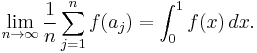
For every Riemann integrable function f on [0, 1],

$\lim_{n\to\infty} \frac{1}{n} \sum_{j=1}^n f(a_j)=\int_0^1 f(x)\, dx.$

For every nonzero integer k,

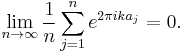
$\lim_{n\to\infty} \frac{1}{n} \sum_{j=1}^n e^{2\pi ik a_j}=0.$

The third condition is known as Weyl's criterion. Together with the formula for the sum of a finite geometric series, the equivalence of the first and third conditions furnishes an immediate proof of the equidistribution theorem.

Metric theorems

Metric theorems describe the behaviour of a parametrised sequence for almost all values of some parameter α: that is, for values of α not lying in some exceptional set of Lebesgue measure zero.

For any sequence of distinct integers b_n, the sequence {b_n α} is equidistributed mod 1 for almost all values of α.^[1]
The sequence {αⁿ} is equidistributed mod 1 for almost all values of α > 1.^[2]

It is not known whether the sequences {eⁿ} or {πⁿ} are equidistributed mod 1. However it is known that the sequence {αⁿ} is not equidistributed mod 1 if α is a PV number.

Well-distributed sequence

A bounded sequence {s₁, s₂, s₃, …} of real numbers is said to be well-distributed on [a, b] if for any subinterval [c, d] of [a, b] we have

$\lim_{n\to\infty}{ \left|\{\,s_{k%2B1},\dots,s_{k%2Bn} \,\} \cap [c,d] \right| \over n}={d-c \over b-a} \,$

uniformly in k. Clearly every well-distributed sequence is uniformly distributed, but the converse does not hold. The definition of well-distributed modulo 1 is analogous.

References

^ See Satz 1, Über eine Anwendung der Mengenlehre auf ein aus der Theorie der säkularen Störungen herrührendes Problem, Felix Bernstein, Mathematische Annalen 71, #3 (September 1911), pp. 417-439, doi:10.1007/BF01456856.
^ Ein mengentheoretischer Satz über die Gleichverteilung modulo Eins, J. F. Koksma, Compositio Mathematica, 2 (1935), pp. 250-258.

L. Kuipers; H. Niederreiter (2006). Uniform Distribution of Sequences. Dover Publishing. ISBN 0-486-45019-8.
L. Kuipers; H. Niederreiter (1974). Uniform Distribution of Sequences. John Wiley & Sons Inc.. ISBN 0-471-51045-9.

External links

Weisstein, Eric W., "Equidistributed Sequence" from MathWorld.